Image Dataset Report

📚 01. Dataset Overview

Created by Zalando to provide a more realistic and challenging image dataset while maintaining the convenient format of the original MNIST.

🔗 Source

70,000

Total Images

10

Clothing Categories

60,000

Training Set (85%)

10,000

Testing Set (15%)

🔍 02. Exploratory Data Analysis (EDA)

Dataset Examples

Original Format: All images in the dataset are in grayscale format and sized exactly 28x28 pixels. They represent 10 distinct types of clothing and accessories.

Class Distribution

Perfectly Balanced: The dataset exhibits an equal distribution across all 10 classes, with exactly 6,000 samples per class in the training set.

* Hover over the bars to see exact sample counts.

📊 Class Similarity Matrix

Top 5 most similar pairs (High Confusion Risk):

Pullover & Coat (Similarity Score: 9.651)
Pullover & Shirt (Similarity Score: 9.478)
Sandal & Sneaker (Similarity Score: 9.432)
Coat & Shirt (Similarity Score: 9.425)
Trouser & Dress (Similarity Score: 9.396)

⚙️ 03. Setup & Preprocessing Pipeline

Resize: Scale images from 28x28 to 224x224 to increase the input resolution required by modern CNN architectures.
Channel Conversion: Convert 1-channel grayscale images to 3-channel RGB format to match standard pre-trained model input shapes.
Normalization: Normalize pixel values using the standard ImageNet values mean=[0.485, 0.456, 0.406] and std=[0.229, 0.224, 0.225] for stability and convergence speed.

# Define transformations for the dataset
transform = transforms.Compose([
    transforms.Resize((224, 224)),
    transforms.Grayscale(num_output_channels=3),
    transforms.ToTensor(),
    transforms.Normalize(mean=[0.485, 0.456, 0.406], std=[0.229, 0.224, 0.225])
])

# Load Training and Testing Datasets
train_dataset = datasets.FashionMNIST(
    root="./data", train=True, download=True, transform=transform
)
test_dataset = datasets.FashionMNIST(
    root="./data", train=False, download=True, transform=transform
)

# Create DataLoaders
train_loader = DataLoader(train_dataset, batch_size=batch_size, shuffle=True)
test_loader = DataLoader(test_dataset, batch_size=batch_size)

🏗️ 04. Model Building Pipeline

💡 Approach: We compare two state-of-the-art architectures for computer vision: Convolutional Neural Networks (CNN) vs. Vision Transformers (ViT).

CNN: DenseNet121

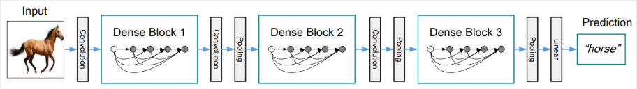
Extracts features hierarchically using dense connectivity patterns, where each layer receives inputs from all preceding layers.

🔗 DenseNet Paper

Vision Transformer (ViT)

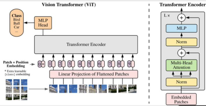
Splits the image into fixed-size patches, linearly embeds them with position encodings, and feeds them into a standard Transformer encoder.

🔗 ViT Paper

🔄 End-to-End Forward Pass & Data Shapes

Below is the data pipeline through the model's stages, detailing the Tensor dimensions (Batch Size is denoted as B) and the semantic meaning of the data at each step.

Raw Image (B, 1, 28, 28)

➔

Preprocessed (B, 3, 224, 224)

➔

Backbone (B, Features)

➔

Class Head Linear(Feat, 10)

➔

Output Logits (B, 10)

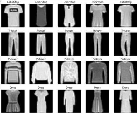
1. Raw Input Image `(B, 1, 28, 28)`

Raw data from the Fashion-MNIST dataset. Each image is a grayscale pixel matrix (1 color channel) with an original size of 28x28 pixels.

2. Preprocessed Tensor `(B, 3, 224, 224)`

Images are resized to 224x224 and duplicated into 3 color channels (RGB) to match the input structure of models pre-trained on ImageNet. Pixel values are normalized to a range of [-1, 1].

3. Backbone Output / Feature Vector `(B, Features)`

The CNN or ViT model acts as a Feature Extractor. The output is a compressed vector containing the high-level semantics of the image.
*For DenseNet121: Features = 1024
*For ViT-Base: Features = 768

4. Classification Head & Output Logits `(B, 10)`

The original classification head (typically 1000 classes) is replaced with a new Fully Connected Layer. It maps the feature vector (1024 or 768 dimensions) down to exactly 10 dimensions corresponding to the 10 clothing/footwear labels. The output values (Logits) are then passed through the Cross-Entropy Loss function to calculate the error during training.

🏆 05. Evaluation & Results

Note: Performance metrics evaluated on the 10,000 unseen test samples.

Model Comparison (Test Set)

Model	Accuracy	Precision	Recall	F1-Score	Params	Inference
DenseNet121	0.9411	0.9411	0.9411	0.9410	~ 6.96M	~ 91.63 ms
ViT-based	0.9064	0.9069	0.9064	0.9054	🏆 ~ 1.32M	⚡ ~ 6.63 ms
Ensemble (Soft Voting)	🏆 0.9454	🏆 0.9456	🏆 0.9454	🏆 0.9454	-	-

🤝 The Ensemble Strategy (Soft Voting)

To achieve the highest performance of 94.54% accuracy, we implemented an Ensemble model using a Soft Voting mechanism. Instead of just taking the final predicted class, we extract the output probability distributions (logits passed through softmax) from both the DenseNet121 and ViT-based models. By averaging these probabilities, the ensemble model effectively combines the hierarchical feature extraction strengths of CNNs with the global context understanding of Vision Transformers, significantly reducing confusion between visually similar classes like Pullover, Coat, and Shirt.

Confusion Matrices

* Click on any matrix to view in full screen.

DenseNet121

ViT-based

Ensemble

Detailed Classification Report

Class	Precision	Recall	F1-Score	Support
0 - T-shirt/top	0.86	0.92	0.88	1000
1 - Trouser	0.99	0.99	0.99	1000
2 - Pullover	0.89	0.94	0.91	1000
3 - Dress	0.91	0.96	0.94	1000
4 - Coat	0.95	0.89	0.92	1000
5 - Sandal	0.99	0.99	0.99	1000
6 - Shirt	0.87	0.76	0.81	1000
7 - Sneaker	0.97	0.98	0.97	1000
8 - Bag	0.99	0.99	0.99	1000
9 - Ankle boot	0.98	0.97	0.97	1000

Class	Precision	Recall	F1-Score	Support
0 - T-shirt/top	0.83	0.87	0.85	1000
1 - Trouser	0.98	0.97	0.98	1000
2 - Pullover	0.84	0.88	0.86	1000
3 - Dress	0.89	0.92	0.90	1000
4 - Coat	0.88	0.85	0.86	1000
5 - Sandal	0.96	0.96	0.96	1000
6 - Shirt	0.78	0.68	0.72	1000
7 - Sneaker	0.94	0.95	0.95	1000
8 - Bag	0.97	0.98	0.97	1000
9 - Ankle boot	0.96	0.94	0.95	1000

Class	Precision	Recall	F1-Score	Support
0 - T-shirt/top	0.88	0.92	0.90	1000
1 - Trouser	0.99	0.99	0.99	1000
2 - Pullover	0.90	0.95	0.92	1000
3 - Dress	0.92	0.97	0.94	1000
4 - Coat	0.96	0.89	0.93	1000
5 - Sandal	0.99	0.99	0.99	1000
6 - Shirt	0.89	0.78	0.83	1000
7 - Sneaker	0.97	0.98	0.98	1000
8 - Bag	0.99	0.99	0.99	1000
9 - Ankle boot	0.98	0.97	0.98	1000

🔬 06. Error Analysis & Interpretability

Common Wrong Predictions

We reviewed images that were frequently mispredicted across the models. We noticed several classes sharing similar visual appearances:

True: Ankle boot ➔ Predict: Sneaker / Sandal
True: Coat ➔ Predict: Pullover / Dress

True: Dress ➔ Predict: T-shirt/top
True: Shirt ➔ Predict: Coat / Dress

Interpretability with Grad-CAM

DenseNet121 - Error Focus

🔍 Key Observations on Model Interpretability

Using Grad-CAM to visualize which regions of the input image contribute most to the prediction, we found that DenseNet121 mainly focuses on the important shape and contour areas of each clothing item instead of irrelevant background information:

👕

T-shirt, Shirt, and Pullover The model correctly pays attention to the upper body area, collars, and sleeve regions to differentiate between these highly similar upper-wear items.
👟

Sandal, Sneaker, and Ankle boot For footwear, the activation maps highlight that the model focuses heavily on the sole and outline/edges to distinguish between open-toe (sandal) and closed-toe (sneaker/boot) designs.

🛡️ 07. Robustness Evaluation (Noise Data)

Although not explicitly detailed in our final report, we conducted robustness experiments by injecting Gaussian noise into the Fashion-MNIST test images. This allowed us to observe how Convolutional architectures (DenseNet) compare to Transformer architectures (ViT) under visual distortion.

import torch

def add_noise(images, std=0.1):
    # Injecting Gaussian noise directly into normalized tensors
    noise = torch.randn_like(images) * std
    noisy_images = images + noise
    
    # Clamp to ensure valid pixel distribution ranges [-1, 1]
    return torch.clamp(noisy_images, -1, 1)

Performance Drop on Noisy Data

Model	Clean Acc (%)	Noisy Acc (%)	Drop (%)
DenseNet121	94.11	~ 84.20	-9.91
ViT-based	90.64	90.03	-0.61
Ensemble	94.54	~ 88.72	-5.82

📌 Conclusion: Transformers (ViT) show remarkable resilience to noise compared to CNNs (DenseNet). While DenseNet relies heavily on local textures and edges (which are easily corrupted by noise), ViT's self-attention mechanism captures global context, allowing it to maintain performance (dropping only 0.61%) even when local pixels are distorted.

🖼️ Image Classification Report