💡 Core Approach: We utilize Contrastive Language-Image Pre-training (CLIP) to perform classification without traditional retraining, applying an aggregated Text Prototype method for Few-shot capabilities.
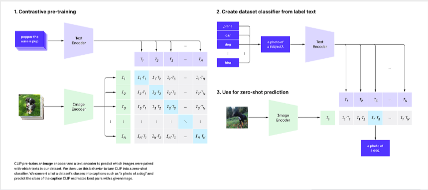
CLIP uses dual encoders (a Vision Transformer for images and a Text Transformer for captions) to map both modalities into a shared, highly semantic multi-dimensional embedding space.
🔄 End-to-End Forward Pass & Prototype Creation
Below is the specialized data pipeline showing how raw data transforms through each stage. Note that tensor dimensions heavily depend on the specific CLIP backbone used (denoted as Res for input resolution and D_feat for feature dimension).
Raw Data
Image (H, W, 3)
Text (Strings)
➔
Preprocessed
Img (1, 3, Res, Res)
Tokens (N_caps, 77)
➔
Encoders
ViT / ResNet
Text Transformer
➔
Embeddings
Img Feat (1, D_feat)
Mean(Txt) ➔ (5, D_feat)
➔
Similarity
Logits (1, 5)
1. Preprocessing (Raw Data ➔ Tensors)
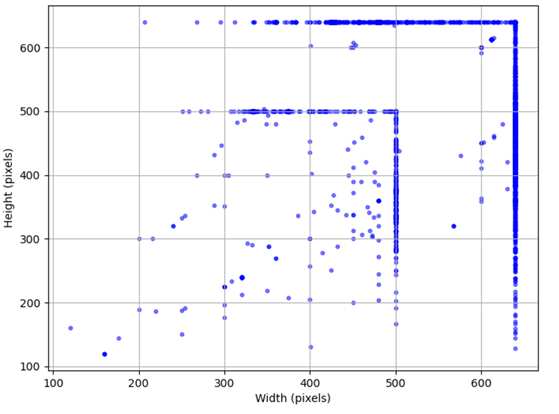
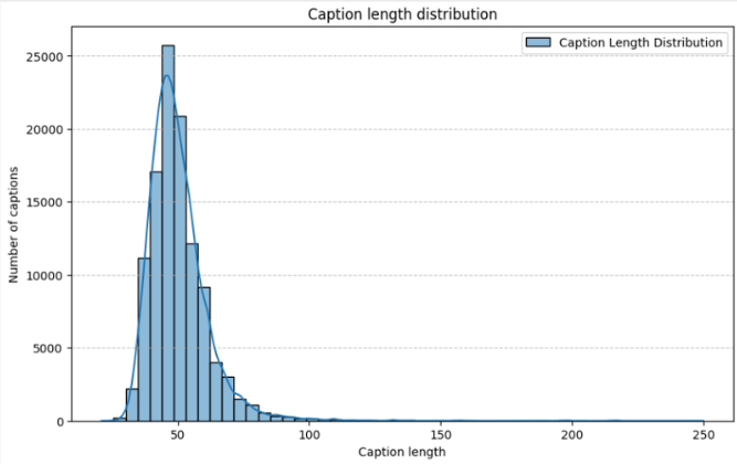
Original images with highly variable sizes (H, W) are first resized and center-cropped by the image preprocessor to a fixed resolution tensor (1, 3, Res, Res) specific to the chosen backbone. Concurrently, raw text captions are tokenized, padded, or truncated to a strictly fixed sequence length of 77 tokens.
| Backbone Architecture |
Input Resolution (Res) |
Feature Dimension (D_feat) |
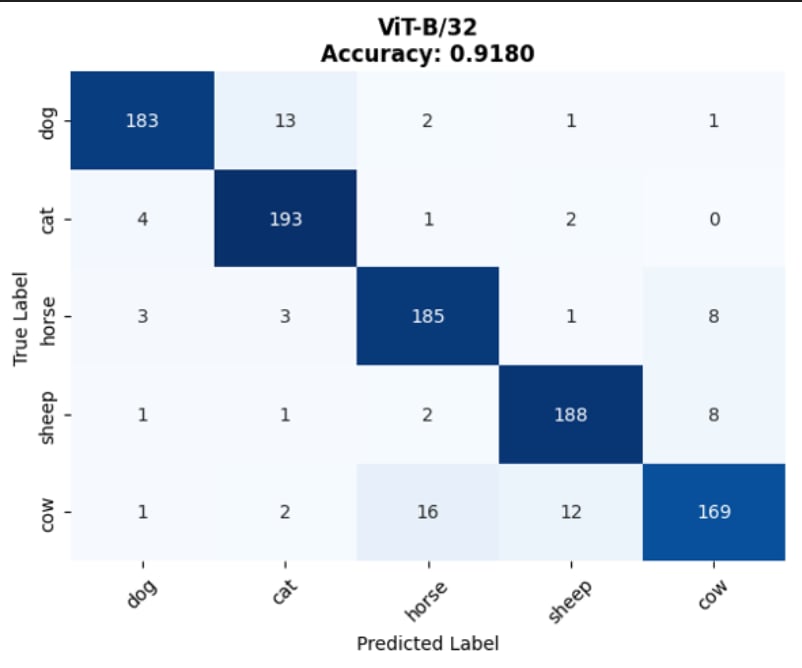
| ViT-B/32 & ViT-B/16 |
224 x 224 |
512 |
| ViT-L/14 |
224 x 224 |
768 |
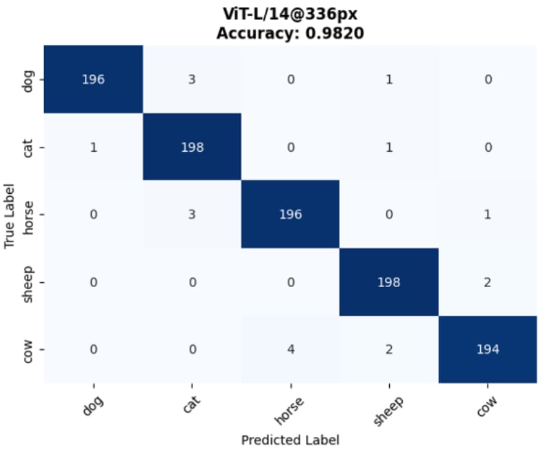
| ViT-L/14@336px |
336 x 336 |
768 |
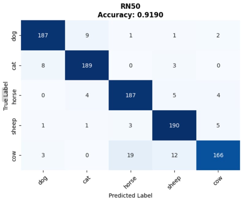
| RN50 |
224 x 224 |
1024 |
| RN50x4 |
288 x 288 |
640 |
| RN50x16 |
384 x 384 |
768 |
2. Text Prototype Aggregation (The Few-Shot Core)
After being processed by the encoders, instead of matching against a single zero-shot prompt ("a photo of a {animal}"), the few-shot model processes all available captions for a class. The resulting text features are L2-normalized, averaged together (Mean Aggregation), and normalized again to form a single, robust Class Prototype vector (5, D_feat).
# 1. Trích xuất đặc trưng (Features) từ Ảnh và Chữ
image_features = model.encode_image(image_input)  # Shape: (1, D_feat)
text_features = model.encode_text(text_inputs)    # Shape: (5, D_feat)

# 2. Chuẩn hóa L2 (L2 Normalization) để đưa về chung không gian độ dài
image_features /= image_features.norm(dim=-1, keepdim=True)
text_features /= text_features.norm(dim=-1, keepdim=True)

# 3. CORE BREAKTHROUGH: Tính Cosine Similarity (Nhân ma trận)
# similarity = (1, D_feat) @ (D_feat, 5) -> (1, 5) Logits
similarity = (100.0 * image_features @ text_features.T).softmax(dim=-1)

# Lấy class có điểm số tương đồng cao nhất
predicted_class = similarity.argmax(dim=-1)
# Create an aggregated representative vector for a class
for c in classes:
    # Extract and normalize text features for all captions of class c
    outputs = model.get_text_features(**inputs)
    text_features = outputs / outputs.norm(dim=-1, keepdim=True)

    # Aggregate N vectors into 1 single prototype via Mean
    class_vector_aggregated = torch.mean(all_text_features, dim=0)

    # Final normalization of the prototype
    class_vector_final = class_vector_aggregated / class_vector_aggregated.norm(dim=-1, keepdim=True)
    class_vectors[c] = class_vector_final
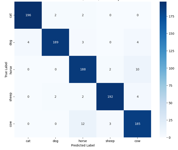
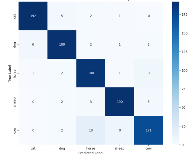
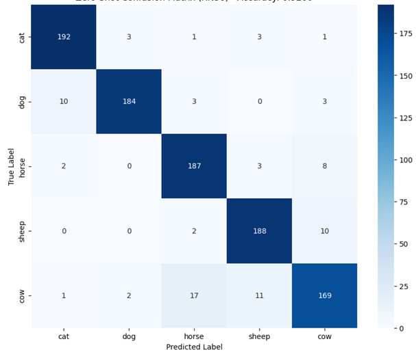
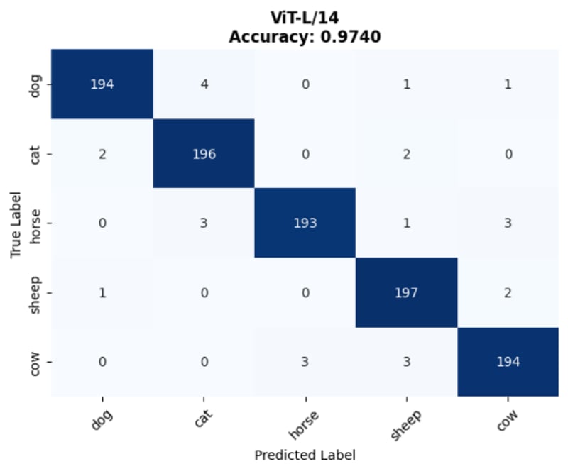
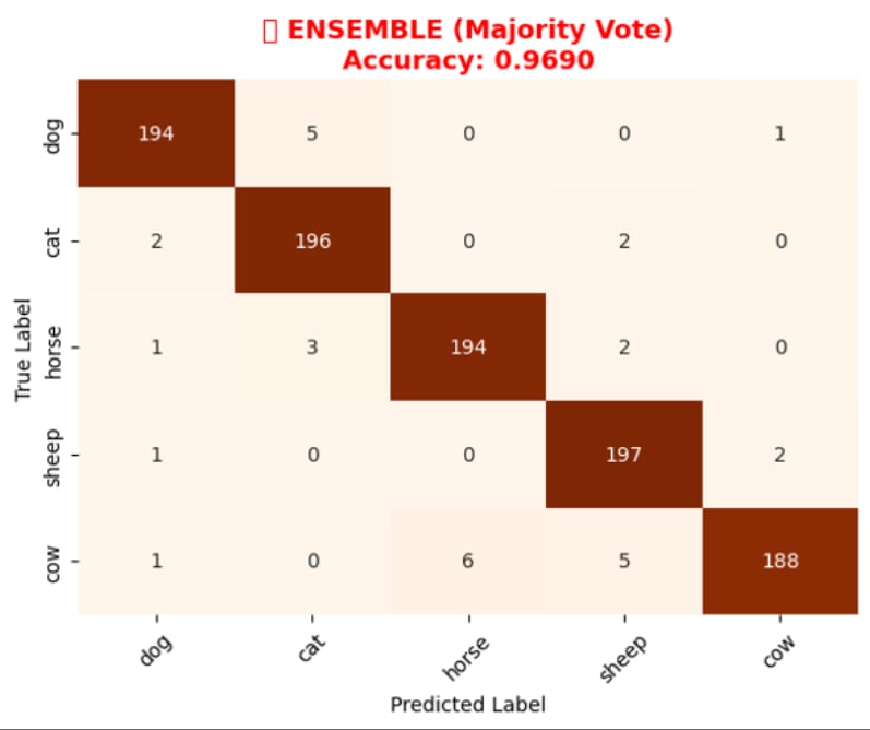
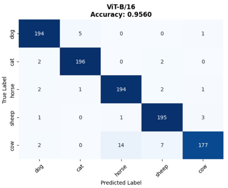
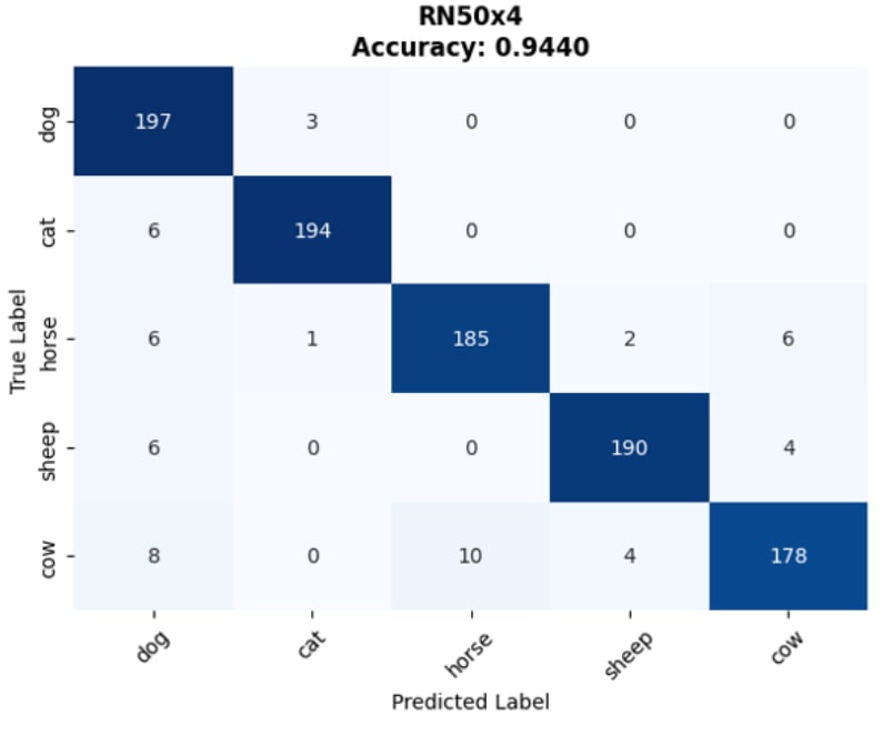
3. Classification via Similarity
When predicting a new image, its extracted feature vector (1, D_feat) is compared against the 5 pre-computed aggregated text prototypes using dot product (Cosine Similarity). The class with the highest similarity score is chosen.